Category Archives: Epidemiology

Covid-19 deaths

I wrote last week about how the number of cases of coronavirus were following a textbook exponential growth pattern. I didn’t look at the number of deaths from coronavirus at the time, as there were too few cases in the UK for a meaningful analysis. Sadly, that is no longer true, so I’m going to take a look at that today.

However, first, let’s have a little update on the number of cases. There is a glimmer of good news here, in that the number of cases has been rising more slowly than we might have predicted based on the figures I looked at last week. Here is the growth in cases with the predicted line based on last week’s numbers.

As you can see, cases in the last week have consistently been lower than predicted based on the trend up to last weekend. However, I’m afraid this is only a tiny glimmer of good news. It’s not clear whether this represents a real slowing in the number of cases or merely reflects the fact that not everyone showing symptoms is being tested any more. It may just be that fewer cases are being detected.

So what of the number of deaths? I’m afraid this does not look good. This is also showing a classic exponential growth pattern so far:

The last couple of days’ figures are below the fitted line, so there is a tiny shred of evidence that the rate may be slowing down here too, but I don’t think we can read too much into just 2 days’ figures. Hopefully it will become clearer over the coming days.

One thing which is noteworthy is that the rate of increase of deaths is faster than the rate of increase of total cases. While the number of cases is doubling, on average, every 2.8 days, the number of deaths is doubling, on average, every 1.9 days. Since it’s unlikely that the death rate from the disease is increasing over time, this does suggest that the number of cases is being recorded less completely as time goes by.

So what happens if the number of deaths continues growing at the current rate? I’m afraid it doesn’t look pretty:

(note that I’ve plotted this on a log scale).

At that rate of increase, we would reach 10,000 deaths by 1 April and 100,000 deaths by 7 April.

I really hope that the current restrictions being put in place take effect quickly so that the rate of increase slows down soon. If not, then this virus really is going to have horrific effects on the UK population (and of course on other countries, but I’ve only looked at UK figures here).

In the meantime, please keep away from other people as much as you can and keep washing those hands.

Covid-19 and exponential growth

One thing about the Covid-19 outbreak that has been particularly noticeable to me as a medical statistician is that the number of confirmed cases reported in the UK has been following a classic exponential growth pattern. For those who are not familiar with what exponential growth is, I’ll start with a short explanation before I move on to what this means for how the epidemic is likely to develop in the UK. If you already understand what exponential growth is, then feel free to skip to the section “Implications for the UK Covid-19 epidemic”.

A quick introduction to exponential growth

If we think of something, such as the number of cases of Covid-19 infection, as growing at a constant rate, then we might think that we would have a similar number of new cases each day. That would be a linear growth pattern. Let’s assume that we have 50 new cases each day, then after 60 days we’ll have 3000 cases. A graph of that would look like this:

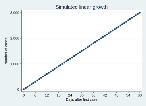
That’s not what we’re seeing with Covid-19 cases. Rather than following a linear growth pattern, we’re seeing an exponential growth pattern. With exponential growth, rather than adding a constant number of new cases each day, the number of cases increases by a constant percentage amount each day. Equivalently, the number of cases multiplies by a constant factor in a constant time interval.

Let’s say that the number of cases doubles every 3 days. On day zero we have just one case, on day 3 we have 2 cases, and day 6 we have 4 cases, on day 9 we have 8 cases, and so on. This makes sense for an infectious disease epidemic. If you imagine that each person who is infected can infect (for example) 2 new people, then you would get a pattern very similar to this. When only one person is infected, that’s just 2 new people who get infected, but if 100 people have the disease, then 200 people will get infected in the same time.

On the face of it, the example above sounds like it’s growing much less quickly than my first example where we have 50 new cases each day. But if you are doubling the number of cases each time, then you start to get to scarily large numbers quite quickly. If we carry on for 60 days, then although the number of cases isn’t increasing much at first, it eventually starts to increase at an alarming rate, and by the end of 60 days we have over a million cases. This is what it looks like if you plot the graph:

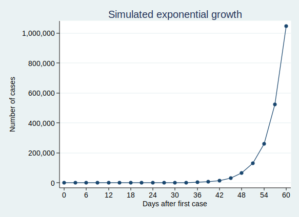
It’s actually quite hard to see what’s happening at the beginning of that curve, so to make it easier to see, let’s use the trick of plotting the number of cases on a logarithmic scale. What that means is that a constant interval on the vertical axis (generally known as the y axis) represents not a constant difference, but a constant ratio. Here, the ticks on the y axis represent an increase in cases by a factor of 10.

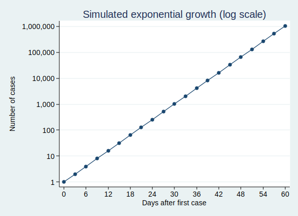
Note that when you plot exponential growth on a logarithmic scale, you get a straight line. That’s because we’re increasing the number of cases by a constant ratio in each unit time, and a constant ratio corresponds to a constant distance on the y axis.

Implications for the UK Covid-19 epidemic

OK, so that’s what exponential growth looks like. What can we see about the number of confirmed Covid-19 cases in the UK? Public Health England makes the data available for download here. The data have not yet been updated with today’s count of cases as I write this, so I added in today’s number (1372) based on a tweet by the Department of Health and Social Care.

If you plot the number of cases by date, it looks like this:

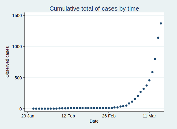
That’s pretty reminiscent of our exponential growth curve above, isn’t it?

It’s worth noting that the numbers I’ve shown are almost certainly an underestimate of the true number of cases. First, it seems likely that some people who are infected will have only very mild (or even no) symptoms, and will not bother to contact the health services to get tested. You might say that it doesn’t matter if the numbers don’t include people who aren’t actually ill, and to some extent it doesn’t, but remember that they may still be able to infect others. Also, there is a delay from infection to appearing in the statistics. So the official number of confirmed cases includes people only after they have caught the disease, gone through the incubation period, developed symptoms that were bothersome enough to seek medical help, got tested, and have the test results come back. This represents people who were infected probably at least a week ago. Given that the number of cases are growing so rapidly, the number of people actually infected today will be considerably higher than today’s statistics for confirmed cases.

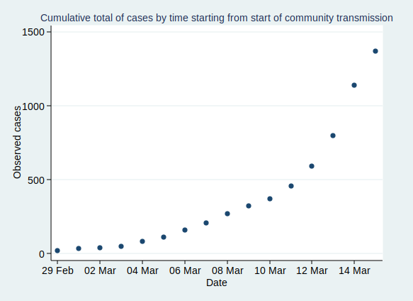
Now, before I get into analysis, I need to decide where to start the analysis. I’m going to start from 29 February, as that was when the first case of community transmission was reported, so by then the disease was circulating within the UK community. Before then it had mainly been driven by people arriving in the UK from places abroad where they caught the disease, so the pattern was probably a bit different then.

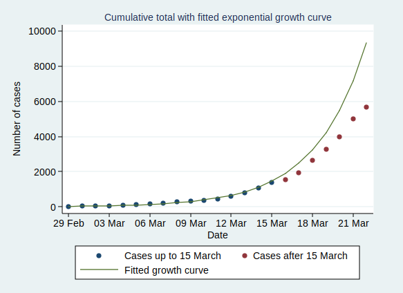
If we start the graph at 29 February, it looks like this:

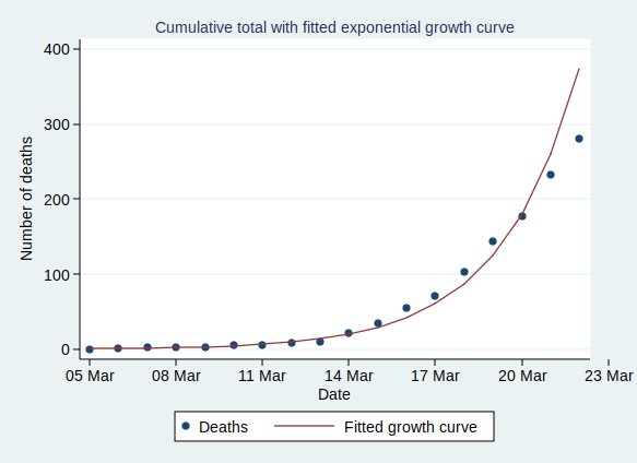
Now, what happens if we fit an exponential growth curve to it? It looks like this:

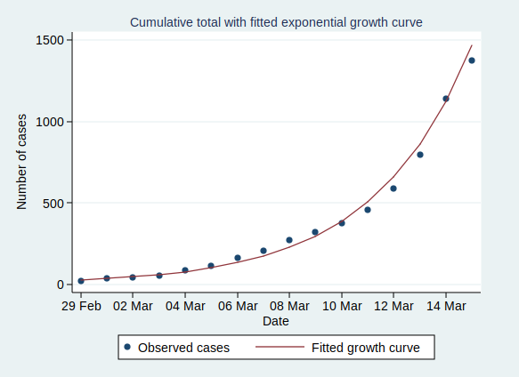
(Technical note for stats geeks: the way we actually do that is with a linear regression analysis of the logarithm of the number of cases on time, calculate the predicted values of the logarithm from that regression analysis, and then back-transform to get the number of cases.)

As you can see, it’s a pretty good fit to an exponential curve. In fact it’s really very good indeed. The R-squared value from the regression analysis is 0.99. R-squared is a measure of how well the data fit the modelled relationship on a scale of 0 to 1, so 0.99 is a damn near perfect fit.

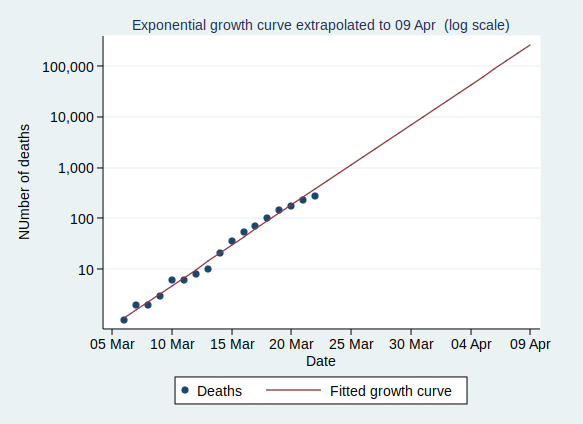
We can also plot it on a logarithmic scale, when it should look like a straight line:
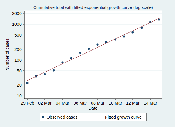
And indeed it does.

There are some interesting statistics we can calculate from the above analysis. The average rate of growth is about a 30% increase in the number of cases each day. That means that the number of cases doubles about every 2.6 days, and increases tenfold in about 8.6 days.

So what happens if the number of cases keeps growing at the same rate? Let’s extrapolate that line for another 6 weeks:

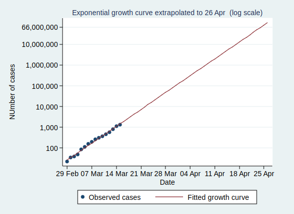
This looks pretty scary. If it continues at the same rate of exponential growth, we’ll get to 10,000 cases by 23 March (which is only just over a week away), to 100,000 cases by the end of March, to a million cases by 9 April, and to 10 million cases by 18 April. By 24 April the entire population of the UK (about 66 million) will be infected.

Now, obviously it’s not going to continue growing at the same rate for all that time. If nothing else, it will stop growing when it runs out of people to infect. And even if the entire population have not been infected, the rate of new infections will surely slow down once enough people have been infected, as it becomes increasingly unlikely that anyone with the disease who might be able to pass it on will encounter someone who hasn’t yet had it (I’m assuming here that people who have already had the disease will be immune to further infections, which seems likely, although we don’t yet know that for sure).

However, that effect won’t kick in until at least several million people have been infected, a situation which we will reach by the middle of April if other factors don’t cause the rate to slow down first.

Several million people being infected is a pretty scary prospect. Even if the fatality rate is “only” about 1%, then 1% of several million is several tens of thousands of deaths.

So will the rate slow down before we get to that stage?

I genuinely don’t know. I’m not an expert in infectious disease epidemiology. I can see that the data are following a textbook exponential growth pattern so far, but I don’t know how long it will continue.

Governments in many countries are introducing drastic measures to attempt to reduce the spread of the disease.

The UK government is not.

It is not clear to me why the UK government is taking a more relaxed approach. They say that they are being guided by the science, but since they have not published the details of their scientific modelling and reasoning, it is not possible for the rest of us to judge whether their interpretation of the science is more reasonable than that of many other European countries.

Maybe the rate of infection will start to slow down now that there is so much awareness of the disease and of precautions such as hand-washing, and that even in the absence of government advice, many large gatherings are being cancelled.

Or maybe it won’t. We will know more over the coming weeks.

One final thought. The government’s latest advice is for people with mild forms of the disease not to seek medical help. This means that the rate of increase of the disease may well appear to slow down as measured by the official statistics, as many people with mild disease will no longer be tested and so not be counted. It will be hard to know whether the rate of infection is really slowing down.

Obesity and dementia

It’s always difficult to draw firm conclusions from epidemiological research. No matter how large the sample size and how carefully conducted the study, it’s seldom possible to be sure that the result you have found is what you were looking for, and not some kind of bias or confounding.

So when I heard in the news yesterday that overweight and obese people were at reduced risk of dementia, my first thought was “I wonder if that’s really true?”

Well, the paper is here. Sadly behind a paywall (seriously guys? You know it’s 2015, right?), though luckily the researchers have made a copy of the paper available as a Word document here.

In many ways, it’s a pretty good study. Certainly no complaints about the sample size: they analysed data on nearly 2 million people. With a median follow-up time of over 9 years, their analysis was based on a long enough time period to be meaningful. They had also thought about the obvious problem with looking at obesity and dementia, namely that obese people may be less likely to get dementia not because obesity protects them against dementia, but just because they are more likely to die of an obesity-related disease before they are old enough to develop dementia.

The authors did a sensitivity analysis in which they assumed that patients who died during the observation period had twice the risk of developing dementia had they lived of patients who survived to the end of follow-up. Although that weakened the negative association between overweight and dementia, it was still present.

There are, of course, other ways to do this. Perhaps it might have been appropriate to use a competing risks survival model instead of the Poisson model they used for their statistical analysis, and if you were going to be picky, you could say their choice of statistical analysis was a bit fishy (sorry, couldn’t resist).

But I don’t think the method of analysis is the big problem here.

For a start, although some of the most obvious confounders (age, sex, smoking, drinking, relevant medication use, diabetes, and previous myocardial infarction) were adjusted for in the analysis, there was no adjustment for socioeconomic status or education level, which is a big omission.

But more importantly, I think the major limitation of these results comes from what is known as the healthy survivor effect.

Let me explain.

The people followed up in the study were all aged over 40 at the start. But there was no upper age limit. Some people were aged over 90 at the start. And not surprisingly, most of the cases of dementia occurred in older people.  Only 18 cases of dementia occurred in those aged 40-44, whereas over 12,000 cases were observed in those aged 80-84. So it’s really the older age groups who are dominating the analysis. Over half the cases of dementia occurred in people aged > 80, and over 90% occurred in people aged > 70.

Now, let’s think about those 80+ year olds for a minute.

There is reasonably good evidence that obese people die younger, on average, than those of normal weight. So the obese people who were aged > 80 at the start of the study are probably not normal obese people. They are probably healthier than average obese people. Many obese people who are less healthy than average would be dead before they are 80, so would never have the chance to be included in that age group of the study.

So in other words, the old obese people in the study are not typical obese people: they are unusually healthy obese people.

That may be because they have good genes or it may be because something about their lifestyle is keeping them healthy, but one way or another, they have managed to live a long life despite their obesity. This is an example of the healthy survivor effect.

There will also be a healthy survivor effect at play in the people of normal weight at the upper end of the age range, but that will probably be less marked, as they haven’t had to survive despite obesity.

I think it is therefore possible that this healthy survivor effect may have skewed the results. The people with obesity may have been at less risk of dementia not because their obesity protected them, but because they were a biased subset of unusually healthy obese people.

This does not, of course, mean that obesity doesn’t protect against dementia. Maybe it does. One thing that would have been interesting would be to see the results broken down by the type of dementia. It is hard to believe that obesity would protect against vascular dementia, when on the whole it is a risk factor for other vascular diseases, but the hypothesis that it could protect against Alzheimer’s disease doesn’t seem so implausible.

What it does mean is that we have to be really careful when interpreting the results of epidemiological studies such as this one. It is always extremely hard to know to what extent the various forms of bias that can creep into epidemiological studies have influenced the results.


Ovarian cancer and HRT

Yesterday’s big health story in the news was the finding that HRT ‘increases ovarian cancer risk’. The scare quotes there, of course, tell us that that’s probably not really true.

So let’s look at the study and see what it really tells us. The BBC can be awarded journalism points for linking to the actual study in the above article, so it was easy enough to find the relevant paper in the Lancet.

This was not new data: rather, it was a meta-analysis of existing studies. Quite a lot of existing studies, as it turns out. The authors found 52 epidemiological studies investigating the association between HRT use and ovarian cancer. This is quite impressive. So despite ovarian cancer being a thankfully rare disease, the analysis included over 12,000 women who had developed ovarian cancer. So whatever other criticisms we might make of the paper, I don’t think a small sample size is going to be one of them.

But what other criticisms might we make of the paper?

Well, the first thing to note is that the data are from epidemiological studies. There is a crucial difference between epidemiological studies and randomised controlled trials (RCTs). If you want to know if an exposure (such as HRT) causes an outcome (such as ovarian cancer), then the only way to know for sure is with an RCT. In an epidemiological study, where you are not doing an experiment, but merely observing what happens in real life, it is very hard to be sure if an exposure causes an outcome.

The study showed that women who take HRT are more likely to develop ovarian cancer than women who don’t take HRT. That is not the same thing as showing that HRT caused the excess risk of ovarian cancer. It’s possible that HRT was the cause, but it’s also possible that women who suffer from unpleasant menopausal symptoms (and so are more likely to take HRT than those women who have an uneventful menopause) are more likely to develop ovarian cancer. That’s not completely implausible. Ovaries are a pretty relevant organ in the menopause, and so it’s not too hard to imagine some common factor that predisposes both to unpleasant menopausal symptoms and an increased ovarian cancer risk.

And if that were the case, then the observed association between HRT use and ovarian cancer would be completely spurious.

So what this study shows us is a correlation between HRT use and ovarian cancer, but as I’ve said many times before, correlation does not equal causation. I know I’ve been moaned at by journalists for endlessly repeating that fact, but I make no apology for it. It’s important, and I shall carry on repeating it until every story in the mainstream media about epidemiological research includes a prominent reminder of that fact.

Of course, it is certainly possible that HRT causes an increased risk of ovarian cancer. We just cannot conclude it from that study.

It would be interesting to look at how biologically plausible it is. Now, I’m no expert in endocrinology, but one little thing I’ve observed makes me doubt the plausibility. We know from a large randomised trial that HRT increases breast cancer risk (at least in the short term). There also seems to be evidence that oral contraceptives increase breast cancer risk but decrease ovarian cancer risk. With my limited knowledge of endocrinology, I would have thought the biological effects of HRT and oral contraceptives on cancer risk would be similar, so it just strikes me as odd that they would have similar effects on breast cancer risk but opposite effects on ovarian cancer risk. Anyone who knows more about this sort of thing than I do, feel free to leave a comment below.

But leaving aside the question of whether the results of the latest study imply a causal relationship (though of course we’re not really going to leave it aside, are we? It’s important!), I think there may be further problems with the study.

The paper tells us, and this was widely reported in the media, that “women who use hormone therapy for 5 years from around age 50 years have about one extra ovarian cancer per 1000 users”.

I’ve been looking at how they arrived at that figure, and it’s not totally clear to me how it was calculated. The crucial data in the paper is this table.  The table is given in a bit more detail in their appendix, and I’m reproducing the part of the table for 5 years of HRT use below.


 Age group  Baseline risk (per 1000)  Relative excess risk Absolute excess risk (per 1000)
 50-54  1.2  0.43  0.52
 55-59  1.6  0.23  0.37
 60-64  2.1  0.05  0.10
 Total  0.99

The table is a bit complicated, so some words or explanation are probably helpful. The baseline risk is the probability (per 1000) of developing ovarian cancer over a 5 year period in the relevant age group. The relative excess risk is the proportional amount by which that risk is increased by 5 years of HRT use starting at age 50. The absolute excess risk is the baseline risk multiplied by the relative excess risk.

The risk in each 5 year period is then added together to give the total excess lifetime risk of ovarian cancer for a woman who takes HRT for 5 years starting at age 50. I assume excess risks at older age groups are ignored as there is no evidence that HRT increases the risk after such a long delay. It’s important to note here that the figure of 1 in 1000 excess ovarian cancer cases refers to lifetime risk: not the excess in a 5 year period.

The figures for incidence seem plausible. The figures for absolute excess risk are correct if the relative excess risk is correct. However, it’s not completely clear where the figures for relative risk come from. We are told they come from figure 2 in the paper. Maybe I’m missing something, but I’m struggling to match the 2 sets of figures. The excess risk of 0.43 for the 50-54 year age group matches the relative risk 1.43 for current users with duration < 5 years (which will be true while the women are still in that age group), but I can’t see where the relative excess risks of 0.23 and 0.05 come from.

Maybe it doesn’t matter hugely, as the numbers in figure 2 are in the same ballpark, but it always makes me suspicious when numbers should match and don’t.

There are some further statistical problems with the paper. This is going to get a bit technical, so feel free to skip the next two paragraphs if you’re not into statistical details. To be honest, it all pales into insignificance anyway beside the more serious problem that correlation does not equal causation.

The methods section tells us that cases were matched with controls. We are not told how the matching was done, which is the sort of detail I would not expect to see left out of a paper in the Lancet. But crucially, a matched case control study is different to a non-matched case control study, and it’s important to analyse it in a way that takes account of the matching, with a technique such as conditional logistic regression. Nothing in the paper suggests that the matching was taken into account in the analysis. This may mean that the confidence intervals for the relative risks are wrong.

It also seems odd that the data were analysed using Poisson regression (and no, I’m not going to say “a bit fishy”). Poisson regression makes the assumption that the baseline risk of developing ovarian cancer remains constant over time. That seems a highly questionable assumption here. It would be interesting to see if the results were similar using a method with more relaxed assumptions, such as Cox regression. It’s also a bit fishy (oh damn, I did say it after all) that the paper tells us that Poisson regression yielded odds ratios. Poisson regression doesn’t normally yield odds ratios: the default statistic is an incidence rate ratio. Granted, the interpretation is similar to an odds ratio, but they are not the same thing. Perhaps there is some cunning variation on Poisson regression in which the analysis can be coaxed into giving odds ratios, but if there is, I’m not aware of it.

I’m not sure how much those statistical issues matter. I would expect that you’d get broadly similar results with different techniques. But as with the opaque way in which the lifetime excess risk was calculated, it just bothers me when statistical methods are not as they should be. It makes you wonder if anything else was wrong with the analysis.

Oh, and a further oddity is that nowhere in the paper are we told the total sample size for the analysis. We are told the number of women who developed ovarian cancer, but we are not told the number of controls that were analysed. That’s a pretty basic piece of information that I would expect to see in any journal, never mind a top-tier journal such as the Lancet.

I don’t know whether those statistical oddities have a material impact on the analysis. Perhaps they do, perhaps they don’t. But ultimately, I’m not sure it’s the most important thing. The really important thing here is that the study has not shown that HRT causes an increase in ovarian cancer risk.

Remember folks, correlation does not equal causation.

Are two thirds of cancers really due to bad luck?

A paper published in Science has been widely reported in the media today. According to media reports, such as this one, the paper showed that two thirds of cancers are simply due to bad luck, and only one third are due to environmental, lifestyle, or genetic risk factors.

The paper shows no such thing, of course.

It’s actually quite an interesting paper, and I’d encourage you to read it in full (though sadly it’s paywalled, so you may or may not be able to). But it did not show that two thirds of cancers are due to bad luck.

What the authors did was they looked at the published literature on 31 different types of cancer (eg lung cancer, thyroid cancer, colorectal cancer, etc) and estimated 2 quantities for each type of cancer. They estimated the lifetime risk of getting the cancer, and how often stem cells divide in those tissues.

They found a very strong correlation between those two quantities: tissues in which stem cells divided frequently (eg the colon) were more likely to develop cancer than tissues in which stem cell division was less frequent (eg the brain).

The correlation was so strong, in fact, that it explained two thirds of the variation among different tissue types in their cancer incidence. The authors argue that because mutations that can lead to cancer can occur during stem cell division purely by chance, that means that two thirds of the variation in cancer risk is due to bad luck.

So, that explains where the “two thirds” figure comes from.

The problem is that it applies only to explaining the variation in cancer risk from one tissue to another. It tells us nothing about how much of the risk within a given tissue is due to modifiable factors. You could potentially see exactly the same results whether each specific type of cancer struck completely at random or whether each specific type were hugely influenced by environmental risk factors.

Let’s take lung cancer as an example. Smoking is a massively important risk factor. Here’s a study that estimated that over half of all lung cancer deaths in Japanese males were due to smoking. Or to take cervical cancer as another example, about 70% of cervical cancers are due to just 2 strains of the HPV virus.

Those are important statistics when considering what proportion of cancers are just bad luck and what proportion are due to modifiable risk factors, but they did not figure anywhere in the latest analysis.

So in fact, interesting though this paper is, it tells us absolutely nothing about what proportion of cancer cases are due to modifiable risk factors.

We often see medical research badly reported in the newspapers. Often it doesn’t matter very much. But here, I think real harm could be done. The message that comes across from the media is that cancer is just a matter of luck, so changing your lifestyle won’t make much difference anyway.

We know that lifestyle is hugely important not only for cancer, but for many other diseases as well. For the media to claim give the impression that lifestyle isn’t important, based on a misunderstanding of what the research shows, is highly irresponsible.

Edit 5 Jan 2015:

Small correction made to the last paragraph following discussion in the comments below. Old text in strikethrough, new text in bold.